FAGE Analysis Pipeline (ver 0.6.2)

1 Analytical Flow of Pipeline

Multi-environmental trial (MET) analyses are critical for plant breeding programs. In MET group of genotypes are evaluated in several environments (sites, years, or treatments) in order to assess their levels of consistency (or stability) of the performance across these different environments. This lack of stability is known as genotype-by-environment (GxE) interaction and is the result of specific gene responses to the particular conditions of a given environment.

Single- versus Two-stage Analysis

For the analyses of MET, ideally all trials should be evaluated by fitting a unique complete model. This is known as single-stage analysis. In here, the original phenotypic measurements from all trials are modeled together and genetic, non-genetic and residuals variances for each trial are estimated. This process can be challenging and often there are computational complications, mostly originating by the large number of variance components to simultaneously estimate.

An alternative to the above approach is to perform a two-stages analysis. This is divided into two steps. In the step 1 each trial is first analyzed individually. Here, all relevant factors, covariates and spatial components are considered, and once a final model is selected, adjusted means (BLUEs) are obtained for each of the genotypes in the trial together with its weights (further details later). Then, in the step 2, all individual trial analyses are combined and used to fit a single linear mixed-model (LMM) that considers weights.

Both the single-stage and two-stages analyses have advantages and disadvantages. The most important advantage of the two-stages analysis is that it allows considering any relevant design or statistical elements for each trial. This includes different aspects such as spatial analyses, replication, etc. It is common for a single-stage analysis to have too much complexity making it difficult or near impossible to fit, and often some model simplifications are required (e.g., dropping some model terms). These simplifications can translate into important losses of accuracy.

Similarly, in the two-stages analyses, there is some loss of information, as the parameter estimation is done in two steps. However, this separation, allows for the first step to have as much complexity as desired, and often better information is obtained from this stage.

There is another important advantage of the two-stages analysis, and this is related to developing operational analytical pipelines. A single-stage analysis requires all the raw data available for the analysis at the moment of fitting the model. In contrast, the two-stages analyses the first step can be executed in advance and this information can be then retrieved to fit a second step with the desired trials and genotypes. This has also the advantage that the adjusted means (and weights) from the first step can be used for other studies such as genomic prediction (GP) and/or genome-wide association studies (GWAS).

Steps of the Two-stage Analysis

The focus on this pipeline will be on the use of two-stage analyses. As indicated earlier, in the first step, the raw phenotypic data of each trial is analyzed. The idea is to use all available statistical tools to fit each of these trials providing the largest possible accuracy on the genotype’s predictions. In the current pipeline, each site is been evaluated considering genotype as a random effect (allowing for the estimation of heritability), and several model terms are considered to control for potential spatial heterogeneity. These include elements such as autoregressive errors or order 1 (AR1) for the rows and columns, polynomials or spline to model trends, random row or column effects nested within replicate also to model trends.

The procedure evaluates several of these models and according to a given criteria (AIC, BIC, heritability) where the best fitted model is selected. If a low heritability is found (threshold specified by the user) then the trials are not considered in the second step of this analysis. Otherwise, the fitting proceeds. Here, all variance component estimates are fixed to their estimates, and the model is refitted with the genotype effect considered as a fixed effect. From here, adjusted means (or BLUE means, or predictions) are obtained for each of the genotypes together with their weights. Weights are obtained as the diagonal of the inverse of the variance-covariance matrix of adjusted mean estimates (or predictions).

It is important to note, that the current pipeline (workflow) also considers a careful exploration of each individual trial fit, where residual plots are checked, outliers are detected (and eliminated) in a semi-automatic way, and several other statistics are available (such as coefficient of variation, CV%) in order to assess the quality of each of these model fits. These fits should be checked carefully, as the predictions obtained will be stored and possibly used for many years and for different statistical evaluations.

For the second step, information from each of the individual fits is collected. This is an important aspect of the workflow, as different sets of trials can be selected for different objectives. For example, only trials from the current year might be evaluated, but also trials from, for example drought years, might be combined into a single two-stage MET analysis.

One important aspect to consider in this stage before proceeding is to check connectivity between trials by auditing the collected data. The MET analysis will not converge if no genotypes are common between some pairs of trials, or if only very few genotypes are common between trials. As a rule of thumb, we recommend having at least 5 genotypes in common. However, note that important levels of unbalanced are often tolerated by LMMs (particularly in factor analytic structures), but still some connectivity is still required.

After this audit, it is possible to fit the LMM with complex structures. Here, the current workflow considers the structures of single correlation and common variance (CORV), single correlation and heterogeneous variances (CORH), and several factor analytic (FA) structures.

The focus of the current pipeline is mainly on the FA structure as this has several advantages such as: 1) greatest model flexibility with approximations to different correlations and heterogeneous variances, 2) straightforward interpretation of some of the components (loadings, specific, etc.), 3) allows for estimation of some correlations even under poor connectivity, 4) less convergency issues than other structures, such as CORGH and US. In addition, this structure allows for a better understanding of the patterns of GxE and some selection of individuals for underlying factors that affect the response, and therefore that induces the observed pattern of GxE effects found in the data.

Further details and illustrations of these steps are presented in the example presented here.

2 Getting Started

There are several R libraries that are used for statistical analyses in the present workflow. The following code specifies which libraries are required, and these will be installed if not available.

• ASReml-R: requires a commercial license to be installed (for further information please check: this)

• QBMS: requires access (login) to the working databases from the BMS system.

The specifications of the analyses are presented in the file config.in that assists on the data manipulations and model fit.

required_packages <- c("QBMS", "asreml", "ggplot2", "lattice", "gridExtra", "dplyr", "plyr", "ggrepel", "tidyr","ggfortify", "missMDA", "ggpubr", "pheatmap", "kableExtra", "DT", "configr", "remotes", "plotly")

not_installed <- required_packages[!(required_packages %in% installed.packages()[ , "Package"])]
if(length(not_installed)) install.packages(not_installed, repos = "http://cran.us.r-project.org")

#if (!require(QBMS)) remotes::install_github("icarda-git/QBMS")
if (!require(bsselectR)) remotes::install_github("walkerke/bsselectR")

# stage-1 required libraries
library(asreml)

## Online License checked out Mon May 20 14:06:58 2024

library(ggplot2)
library(lattice)
library(gridExtra)
library(dplyr)
library(plyr)
library(QBMS)
library(plotly)

# stage-2 extra required libraries
library(ggrepel)
library(tidyr)     # required for reshaping long to wide table of data
library(ggfortify) # required by the ./lib/GBiplot.R
library(missMDA)   # required by the ./lib/GBiplot.R
library(ggpubr)    # get_legend
library(pheatmap)  # pretty heatmap!

# r markdown required libraries
library(kableExtra)
library(DT)
library(configr)
library(bsselectR)

# stage-1 required includes
source("./lib/bms_import.R")
source("./lib/detect_outliers.R")
source("./lib/mcomp_asreml.R")
source("./lib/gral_stats.R")
source("./lib/gral_single_wgt.R")
source("./lib/spatial_selector.R")
source("./lib/fieldmap.R")

# stage-2 required includes
source("./lib/auditMET.R")
source("./lib/stageMET.R")
source("./lib/GBiplot.R")
source("./lib/fa_plots.R")

# get model definitions
load(file = "./lib/MODLIST.Rda")

# remove previouse analysis outputs/plots
unlink("outputs/*", force = TRUE)
unlink("plots/*", force = TRUE)

config_file <- "config.ini"

if (!file.exists(config_file)) {
  warning(paste(config_file, "not exists!"))
  knitr::knit_exit()
}

config <- read.config(file = config_file)

cat(readLines(config_file), sep = '\n')

## [default]
## study.name  = Study
## trait.name  = GY_Calc_kgha
## source.bms  = FALSE
## both.stages = TRUE
## 
## [bms]
## ; define extra params required by BMS API to retrieve the data
## url     = https://bms.icarda.org/ibpworkbench/
## crop    = wheat
## program = Wheat International Nurseries
## 
## [outliers]
## threshold.start = 4
## threshold.stop  = 3
## threshold.step  = 0.25
## 
## [met]
## heritVC.limit = 0.10
## Pvalue.limit  = 0.10
## excluded.loc  = loc_17, loc_09
## excluded.geno = geno_02, geno_11, geno_16, geno_20
## 
## best.fa =

3 Import and Loading Data

In this section we will be importing raw data directly from BMS. However, a standalone file with raw data can also be read and accessed.

# the trial and trait names (e.g., IDYT39 and GY_Calc_kgha respectively)
study.name <- config$default$study.name
trait.name <- config$default$trait.name

3.1 Import from BMS

If you are importing data from BMS (i.e., source.bms is TRUE), then study.name (e.g., “Study”) should exist in the following bms.program in your bms.crop. Also, the trait.name (e.g., “GY_Calc_kgha”) should match your BMS ontology and has observed data. Please check these settings in the associated config file here.

This analysis pipeline is using the QBMS R package to query the Breeding Management System database (using BrAPI calls) and retrieves experiments data directly into R statistical analyzing environment.

You will get a login pop-up window, use the your BMS credentials

# BMS is your data source?
source.bms <- (config$default$source.bms == "TRUE")

# define extra params required by BMS API to retrieve the data
bms.url     <- config$bms$url
bms.crop    <- config$bms$crop
bms.program <- config$bms$program

3.2 Import from Other Sources

If you are reading data directly, then two CSV files are required here in the same directory of this script named as the following:

• Study_germplasm.csv for your list of germplasms, it should contain two columns germplasmName and check (0 for test entries and 1 for check/control entries).

• Study_GY_Calc_kgha_data.csv for your trials data. Mandatory columns are trial, gen (genotypes, they should match with the ones in the previous germplasm list), block (replication), ibk (incomplete blocks), col and row (field layout), and resp (trait response).

If no block (replication) is considered in the designs, this should be filled with a 1 in the dataset. Also, if no ibk (incomplete blocks), column or row coordinates are available, these should be provided as NA in the dataset.

Get the name of required input files and check if they exist:

if(source.bms){
  # data will extracted directly from BMS server and save in intermediate csv files
  files <- bms_import(study.name, trait.name, bms.crop, bms.program, bms.url)
  geno_file <- files$germplasm
  data_file <- files$data
}else{
  # setup the expected names 
  geno_file <- paste0(study.name, "_germplasm.csv")
  data_file <- paste0(study.name, "_", trait.name, "_data.csv")
}

if (!file.exists(data_file)) {
  warning(paste(data_file, "not exists!"))
  knitr::knit_exit()
}
if (!file.exists(geno_file)) {
  warning(paste(geno_file, "not exists!"))
  knitr::knit_exit()
}

3.3 Check for Mandatory Columns

The following code is an internal check that the required columns are provided in their respective data frames.

# load data 
data <- read.csv(data_file)
germplasm.data <- read.csv(geno_file)

if("studyId" %in% colnames(data)) {
  bms.studyId  <- data$studyId[1]
  data$studyId <- NULL
}

# QC: check for mandatory columns
oops <- setdiff(c("trial", "gen", "block", "ibk", "col", "row", "resp"), colnames(data))
if(length(oops) > 0) {
  warning(paste("Can't find the following mandatory columns in your data file", 
                data_file, "\n", paste(oops,  collapse = ", ")))
  knitr::knit_exit()
}

oops <- setdiff(c("germplasmName", "check"), colnames(germplasm.data))
if(length(oops) > 0) {
  warning(paste("Can't find the following mandatory columns in your germplasm file", 
                geno_file, "\n", paste(oops, collapse = ", ")))
  knitr::knit_exit()
}

3.4 Data Pre-processing

In this section, some conversions of columns within a data frame are performed to be ready for the downstream analyses (e.g., convert to factor, sorting, and unique identifier).

# make sure that design and experimental treatments are factors, and response is numeric
data$gen   <- factor(data$gen)
data$trial <- factor(data$trial)
data$block <- factor(data$block)
data$ibk   <- factor(data$ibk)
data$col   <- factor(data$col)
data$row   <- factor(data$row)
data$resp  <- as.numeric(as.character(data$resp))

# you MUST sort your data into the order you specify in the rcov/residuals term
data <- data[with(data, order(trial, row, col)),]

# create a unique record identifier
data$id <- 1:dim(data)[1]

3.5 Extract Check Entries

Extract the names of check entries and tag them in the data file:

It is important to verify that these entries are the ones defined as checks (or controls).

# germplasm list has a column refers if any entry is test(0) or check(1)
check.name <- germplasm.data$germplasmName[germplasm.data$check == 1]

# create check column (handle weird cases like extra spaces and/or uppercase/lowercase letters!)
data$check <- ifelse(gsub(" ","",tolower(data$gen)) %in% gsub(" ","",tolower(check.name)), 1, 0)

Check entries are: geno_02, geno_11, geno_16, geno_20

3.6 Define Experimental Design

Define the type of experiment design for each trial and assess the availability of spatial information. The available designs in this pipeline are:

• ALPHA: alpha-lattice design.
• RCBD: randomized complete block design.
• AUGMENTED: RCBD augmented design in a RCBD.
• PREP: partially-replicated design.

# create a new data.frame to report all issues related to the row/col data if there is any
spatial.issues <- data.frame("trial" = character(), "issue" = character(), 
                             "row" = character(), "col" = character())

# create a new data.frame list experiment design of each trial (ALPHA, RCBD, AUGMENTED, PREP)
trial.type <- data.frame("trial" = character(), stringsAsFactors = FALSE)

#***************************************
#* Design       has.block     has.ibk
#* 
#* CRD          FALSE         FALSE
#* AUGMENTED    FALSE         TRUE
#* RCBD         TRUE          FALSE
#* ALPHA        TRUE          TRUE
#***************************************

# can guess experiment design depends on presence/absence of block and ibk (i.e., rep and block) design factors
for(i in 1:nlevels(data$trial)){
  site.data <- subset(data, trial == levels(data$trial)[i])
  trial.type[i, "trial"]  <- levels(data$trial)[i]

  has.block <- !anyNA(site.data$block) && length(unique(site.data$block)) > 1
  has.ibk   <- !anyNA(site.data$ibk)   && length(unique(site.data$ibk))   > 1

  trial.type[i, "design"] <- ifelse(has.block, 
                                    ifelse(has.ibk, "ALPHA", "RCBD"), 
                                    ifelse(has.ibk, "AUGMENTED", "CRD"))

  has.spatial <- !(anyNA(site.data$row) | anyNA(site.data$col))
  
  if (has.spatial) {
    # assure the row/column data contiguity in the full field dimensions
    contiguous.data <- expand.grid(unique(site.data$row), unique(site.data$col))
    colnames(contiguous.data) <- c("row", "col")
    missing.coords <- setdiff(contiguous.data, site.data[,c("row", "col")])
    
    if (!empty(missing.coords)) {
      missing.coords$issue <- "missing row x col"
      missing.coords$trial <- trial.type[i, "trial"]
      spatial.issues <- rbind(spatial.issues, missing.coords)
    }
    
    # check if there is any duplicate row/col coordinates
    duplicated.coords <- site.data[duplicated(site.data[,c("row", "col")]),]
    
    if (!empty(duplicated.coords)) {
      duplicated.coords <- duplicated.coords[,c("row", "col")]
      duplicated.coords$issue <- "duplicated row x col"
      duplicated.coords$trial <- trial.type[i, "trial"]
      
      spatial.issues <- rbind(spatial.issues, duplicated.coords)
    }
    
    trial.type[i, "has.spatial"] <- paste0("Yes (", length(unique(site.data$row)), "x", 
                                          length(unique(site.data$col)), " row/col)")
    
  } else {
    trial.type[i, "has.spatial"] <- "NO"
  }
}

create_dt(trial.type)

if (!empty(spatial.issues)) {
  warning("has some issues in spatial data integrity!")
  create_dt(spatial.issues)
}

Warning has some issues in spatial data integrity!

3.7 Field Maps

The following code provides a field map to assess the spatial distribution of the response variable for each trial with available spatial information. This is recommended in order to identify potential outliers, trait patterns in the field, potential post-blocking, etc.

# draw fieldmaps!
field.plots <- list()
plot.names  <- list()

for(i in 1:nlevels(data$trial)){
  site.data <- subset(data, trial == levels(data$trial)[i])
  if (anyNA(site.data$row) | anyNA(site.data$col)) next
  field.plots[[i]] <- fieldmap(x=site.data, column="resp", textColumn="gen", asFactor=F, 
                               rows="row", ranges="col", borderColumns="ibk", 
                               main=paste(levels(data$trial)[i], trait.name))
  
  plot.names[[i]] <- levels(data$trial)[i]
  png(paste0("plots/fieldmap_", plot.names[[i]], "_", trait.name, ".png"))
  print(field.plots[[i]])
  dev.off()
}

if (length(plot.names) != 0) {
  field.plots[sapply(field.plots, is.null)] <- NULL
  plot.names[sapply(plot.names, is.null)] <- NULL
  
  pages <- marrangeGrob(grobs = field.plots, nrow=1, ncol=1)
  
  page.width  <- 2 * max(as.numeric(data$col))
  page.height <- 5 * max(as.numeric(data$row))
  
  ggsave(paste0("outputs/", study.name, "_", trait.name, "_Stage-1_Fieldmap.pdf"), 
         plot = pages, width = page.width, height = page.height, dpi = 600, units = "cm", limitsize = FALSE)
  
  select.plot <- paste0("plots/fieldmap_", plot.names, "_", trait.name, ".png")
  names(select.plot) <- plot.names
  bsselect(select.plot, type = "iframe", live_search = TRUE, show_tick = TRUE, elementId = "fieldmaps")$prepend[[1]]$html
} else {
  message("There is no spatial data!")
}

loc_01 loc_02 loc_03 loc_04 loc_05 loc_06 loc_07 loc_08 loc_09 loc_10 loc_11 loc_12 loc_13 loc_14 loc_15 loc_16 loc_17 loc_18 loc_19 loc_20 loc_21

Check your field maps here

4 Single-Environment Analysis

This is the first step of the two-stages analyses where each trial (or environment) is evaluated individually to obtain the ‘best’ possible fit for the trial under study.

4.1 Basic Distribution Plots

These plots highly potential differences in the data that might affect the analyses and should alert the users. These plots assist identifying trials/individuals with large variations or large differences between replications/blocks.

par(mar = c(10, 4, 2, 2) + 0.1)
xyplot(resp ~ gen | trial, groups = block, data = data, 
       scales = list(draw = FALSE), strip = strip.custom(par.strip.text = list(cex = 0.8)))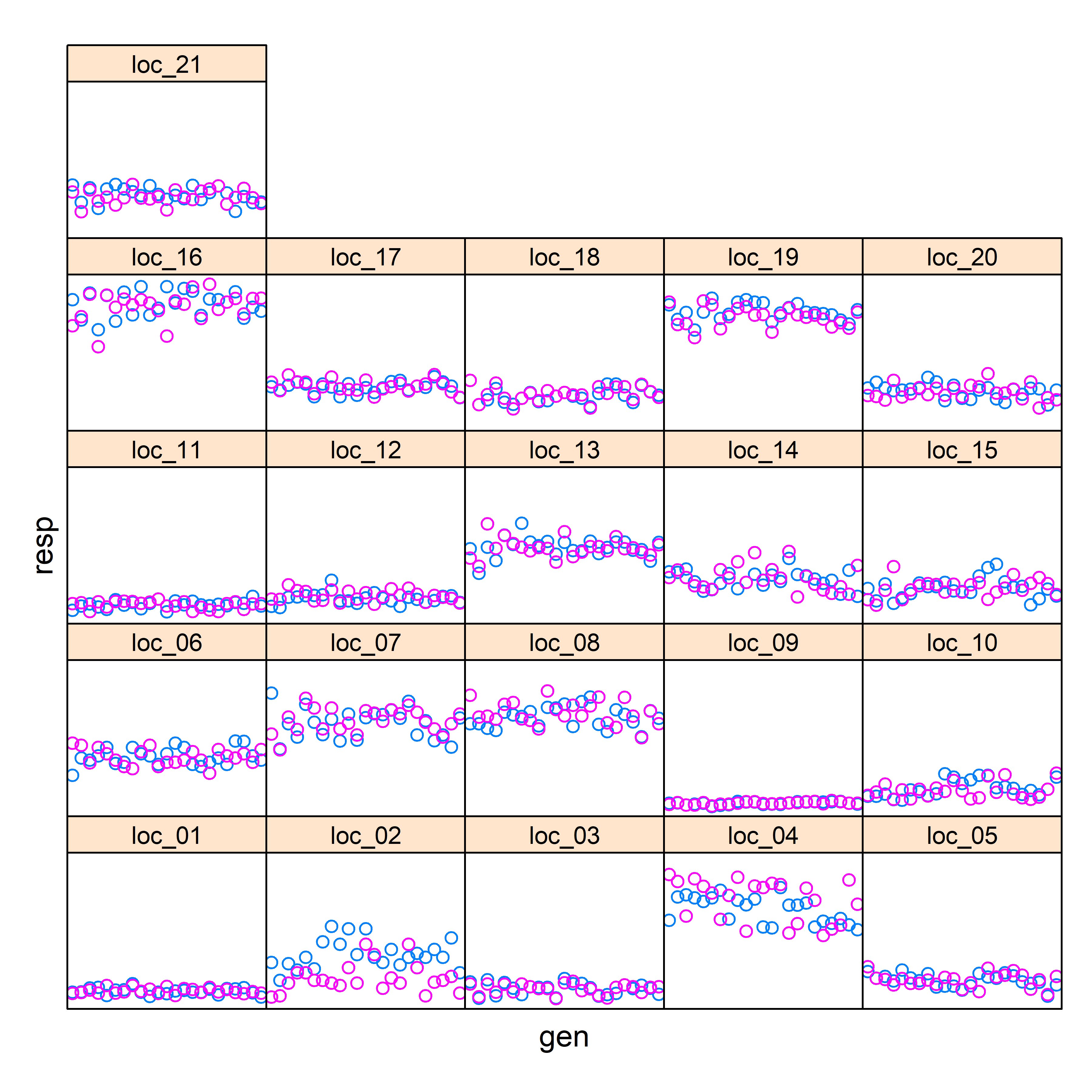

plot_ly(data, y = ~resp, x = ~trial, type = "box", width = 800, height = 480)

plot_ly(data, y = ~resp, x = ~gen, type = "box", width = 800, height = 480)

4.2 Summary Table of Data

• Environment: Environment/location name.
• Type: Experiment design.
• nRep: Number of replications.
• nTotalEntries: Total Number of entries (genotypes).
• nCheckEntries: Total Number of check entries.
• nTestEntries: Total Number of test entries.
• nonNA_nVar: Total Number of non-missing entries.
• nonNA_obs: Total Number of non-missing observations.
• nonNA_AvRep: Average Number of replications for non-missing entries.
• grandMean: Grand mean mu.
• checksMean: Checks mean mu(c).
• newEntriesMean: New entries mean mu(L).
• Trait: Response trait name.
• NumMissing: Number of missing values.
• Min: Minimum value of response.
• Max: Maximum value of response.
• Range: Range of response values.
• Median: Median response value.
• LowerQuartile: Lower Quartile value (25%).
• UpperQuartile: Upper Quartile value (75%).
• MeanRep: Average number of replications.
• MinRep: Minimum number of replications.
• MaxRep: Maximum number of replications.

create_dt(summS[,c(1:12, 19:20, 24:32)])

4.3 Detecting Outliers

These are the residuals and variograms from each trial available to identify potential outliers (scres correspond to the standardized conditional residuals). The interactive graphs are presented below for exploration. However, in addition, some outliers are reported in the database based on the pre-specified thresholds (see table below). Note that some are identified as such (outlier = 1), and counterpart observations (outlier = 0) for the same germplasms in other replications. Close exploration of this database should ensure that the corresponding observations are eliminated.

select.environment <- summS[!is.na(summS$sel_model) & !is.na(summS$residualVar), "Environment"]
select.residual    <- paste0("plots/residual_", select.environment, "_", trait.name, ".png")

names(select.residual) <- select.environment

bsselect(select.residual, 
         type = "iframe", 
         live_search = TRUE, 
         show_tick = TRUE, 
         elementId = 'residuals')$prepend[[1]]$html

loc_01 loc_02 loc_03 loc_04 loc_05 loc_06 loc_07 loc_08 loc_09 loc_10 loc_11 loc_12 loc_13 loc_14 loc_15 loc_16 loc_17 loc_18 loc_19 loc_20 loc_21

select.environment <- summS[!is.na(summS$sel_model) & !is.na(summS$residualVar), "Environment"]
select.variogram   <- paste0("plots/variogram_", select.environment, "_", trait.name, ".png")

names(select.variogram) <- select.environment

bsselect(select.variogram, 
         type = "iframe", 
         live_search = TRUE, 
         show_tick = TRUE, 
         elementId = "variograms")$prepend[[1]]$html

loc_01 loc_02 loc_03 loc_04 loc_05 loc_06 loc_07 loc_08 loc_09 loc_10 loc_11 loc_12 loc_13 loc_14 loc_15 loc_16 loc_17 loc_18 loc_19 loc_20 loc_21

select.environment <- summS[!is.na(summS$sel_model) & trial.type$has.spatial != "NO" & !is.na(summS$residualVar), "Environment"]
select.residual    <- paste0("plots/res_layout_", select.environment, "_", trait.name, ".png")

names(select.residual) <- select.environment

if (length(select.environment) != 0) {
  bsselect(select.residual, 
           type = "iframe", 
           live_search = TRUE, 
           show_tick = TRUE, 
           elementId = 'res_layouts')$prepend[[1]]$html
}

loc_01 loc_02 loc_03 loc_04 loc_05 loc_06 loc_07 loc_08 loc_09 loc_10 loc_11 loc_12 loc_13 loc_14 loc_15 loc_16 loc_17 loc_18 loc_19 loc_20 loc_21

create_dt(temp)

• Description of graphical/numerical step 1 output:
  • residual.plots: Residual plots.
  • variogram.plots: Variogram fitted model.

Check your residual plots here

Check your variogram fitted model here

Check your residual layouts here

4.4 Summary Table of Final Models

The following table presents a summary of the final models selected for each of the individual trials. The final model were fitted after the elimination of outliers (outlier = 1). The procedure in this case fits a total of 26 different spatial models (only 8 in case of Augmented design trials) and selects the best model according to the specified criteria.

It is critical to explore this output database, as from here some of the trials with poor performance (e.g., heritVC < 0.10) should be eliminated as they might have installing or phenotypic issues and therefore they are unlikely to contribute to the downstream MET analyses. This summary table has several relevant statistics that can be used in combination to assess their quality.

• Environment: Environment/location name.
• sel_model: Selected model (see next section).
• heritVC: The heritability calculated based on variance components.
• heritPEV: The heritability calculated based on the predictor error variance (only for genotypes considered as random).
• genotypicVar: Genotypic Variance.
• residualVar: Residual Variance.
• CV: Coefficient of Variation.
• LSD: Least Significant Difference.
• Variance: Total Variance of the response variable.
• SD: Response Standard Deviation.
• WaldStatistic: Wald Chi-Squared Test statistic (mixed model ANOVA-like table).
• WaldDF: Wald-test Degree of Freedom.
• Pvalue: p-value for the test line.

create_dt(summS[,c(1, 13:18, 21:23, 33:35)])

4.5 Models Selection

The table below presents the final models selected according to the criteria specified earlier. The model specifications presented here are just informative, but they provide an idea of the relevance of some model terms in the particular dataset selected.

• Spatial Model selector
  • Model: A numeric value with the number of the selected Model from the list of evaluated models.
  • RepRow: If TRUE the factor for random effects of row (or row within replicated if replicate is available) will be added to the model.
  • RepCol: If TRUE the factor for random effects of column (or column within replicated if replicate is available) will be added to the model.
  • splineRow: If TRUE the factor for random effects of spline for row together with a fixed effect covariate for row will be added to the model.
  • splineCol: If TRUE the factor for random effects of spline for column together with a fixed effect covariate for column will be added to the model.
  • Resid: A string with the specification of type of residual terms to fit. Options are: ‘indep’ and ‘ar1’ for independent errors, and autoregressive of order 1 for both rows and columns.
  • Nugget: If TRUE a nugget random effect (only for autoregressive errors) will be added to the model.
  • List: A numeric value indicating the list category (or priority) to be used to subset the list of evaluated models.
• Non-spatial model selector
• Fitting Criteria

if (length(select.environment) != 0) {
  create_dt(merge(summS[,c("Environment", "sel_model")], 
                  mod.list, 
                  by.x = "sel_model", 
                  by.y = "Model", 
                  sort = FALSE))
} else {
  warning("There is no spatial data!")
}

4.6 Obtaining Predictions

This table is the main output table generated from the first step analyses, where the adjusted means (BLUEs), are obtained from the first step analysis, they need to be stored for further use, as these single-site analyses will not need to be redone in the future.

• gen: Genotype name.
• predicted.value: Predicted response value (BLUEs).
• std.error: Standard Error of predicted value.
• status: A comment to indicate if this predicted value is estimable.
• weight: The inverse of standard error.
• Environment: Environment name.

create_dt(predS)

4.7 BMS Output

folder.name <- paste0("BMS_", format(Sys.Date(), "%Y-%m-%d"), "T", format(Sys.time(), "%H-%M-%S"))

if ("TRIAL_INSTANCE" %in% colnames(data)) {
  dir.create(paste0("./outputs/", folder.name))
  
  col.mean <- paste0(trait.name, "_Means")
  col.se   <- paste0(trait.name, "_UnitErrors")
  
  BMSOutput <- data.frame(matrix(ncol = 6, nrow = dim(predS)[1]))
  colnames(BMSOutput) <- c("TRIAL_INSTANCE", "LOCATION_NAME", "ENTRY_NO", "GID", col.mean, col.se)
  
  lookup.TRIAL_INSTANCE <- unique(data[,c("trial", "TRIAL_INSTANCE")])
  bms.predS  <- merge(predS, lookup.TRIAL_INSTANCE, by.x = "Environment", by.y = "trial", all.x = TRUE)
  
  lookup.germplasm <- germplasm.data[,c("germplasmName", "germplasmDbId", "entryNumber")]
  lookup.germplasm$germplasmName <- gsub(" ","",tolower(lookup.germplasm$germplasmName))
  lookup.germplasm <- lookup.germplasm[!duplicated(lookup.germplasm$germplasmName),]
  bms.predS$gen <- gsub(" ","",tolower(bms.predS$gen))
  
  bms.predS  <- merge(bms.predS, lookup.germplasm, by.x = "gen", by.y = "germplasmName", all.x = TRUE)
  
  bms.predS  <- bms.predS[with(bms.predS, order(Environment, gen)),]
  
  
  BMSOutput$TRIAL_INSTANCE <- bms.predS$TRIAL_INSTANCE
  BMSOutput$LOCATION_NAME  <- bms.predS$Environment
  BMSOutput$ENTRY_NO       <- bms.predS$entryNumber
  BMSOutput$GID            <- bms.predS$germplasmDbId
  BMSOutput[,c(col.mean)]  <- bms.predS$predicted.value
  BMSOutput[,c(col.se)]    <- bms.predS$std.error
  
  write.csv(BMSOutput, paste0("./outputs/", folder.name, "/BMSOutput.csv"), row.names = FALSE)
  
  BMSSummary <- data.frame(matrix(ncol = 28, nrow = dim(summS)[1]))
  colnames(BMSSummary) <- c("TRIAL_INSTANCE", "LOCATION_NAME", "Trait", "NumValues", 
                            "NumMissing", "Mean", "Variance", "SD", "Min", "Max", "Range", 
                            "Median", "LowerQuartile", "UpperQuartile", "MeanRep", "MinRep", 
                            "MaxRep", "MeanSED", "MinSED", "MaxSED", "MeanLSD", "MinLSD", 
                            "MaxLSD", "CV", "Heritability", "WaldStatistic", "WaldDF", "Pvalue")
  
  bms.summS  <- merge(summS, lookup.TRIAL_INSTANCE, by.x = "Environment", by.y = "trial", all.x = TRUE)
  
  BMSSummary$TRIAL_INSTANCE  <- bms.summS$TRIAL_INSTANCE
  BMSSummary$LOCATION_NAME   <- bms.summS$Environment
  BMSSummary$Trait           <- bms.summS$Trait
  BMSSummary$NumValues       <- bms.summS$nonNA_obs
  BMSSummary$NumMissing      <- bms.summS$NumMissing
  BMSSummary$Mean            <- bms.summS$grandMean
  BMSSummary$Variance        <- bms.summS$Variance
  BMSSummary$SD              <- bms.summS$SD
  BMSSummary$Min             <- bms.summS$Min
  BMSSummary$Max             <- bms.summS$Max
  BMSSummary$Range           <- bms.summS$Range
  BMSSummary$Median          <- bms.summS$Median
  BMSSummary$LowerQuartile   <- bms.summS$LowerQuartile
  BMSSummary$UpperQuartile   <- bms.summS$UpperQuartile
  BMSSummary$MeanRep         <- bms.summS$MeanRep
  BMSSummary$MinRep          <- bms.summS$MinRep
  BMSSummary$MaxRep          <- bms.summS$MaxRep
  BMSSummary$MeanSED         <- merge(bms.summS$Environment, 
                                      aggregate(std.error~Environment, data = predS, mean, na.rm = TRUE), 
                                      by = 1, all.x = TRUE)$std.error
  BMSSummary$MinSED          <- merge(bms.summS$Environment, 
                                      aggregate(std.error~Environment, data = predS, min, na.rm = TRUE), 
                                      by = 1, all.x = TRUE)$std.error
  BMSSummary$MaxSED          <- merge(bms.summS$Environment, 
                                      aggregate(std.error~Environment, data = predS, max, na.rm = TRUE), 
                                      by = 1, all.x = TRUE)$std.error
  BMSSummary$MeanLSD         <- bms.summS$LSD
  BMSSummary$MinLSD          <- merge(bms.summS$Environment, 
                                      aggregate(std.error~Environment, data = predS, min, na.rm = TRUE), 
                                      by = 1, all.x = TRUE)$std.error * 1.96
  BMSSummary$MaxLSD          <- merge(bms.summS$Environment, 
                                      aggregate(std.error~Environment, data = predS, max, na.rm = TRUE), 
                                      by = 1, all.x = TRUE)$std.error * 1.96
  BMSSummary$CV              <- bms.summS$CV
  BMSSummary$Heritability    <- bms.summS$heritVC
  BMSSummary$WaldStatistic   <- bms.summS$WaldStatistic
  BMSSummary$WaldDF          <- bms.summS$WaldDF
  BMSSummary$Pvalue          <- bms.summS$Pvalue
  
  write.csv(BMSSummary, paste0("./outputs/", folder.name, "/BMSSummary.csv"), row.names = FALSE)
  
  con <- file(paste0("./outputs/", folder.name, "/BMSInformation.txt.txt"))
  writeLines(c(paste0("InputDataSetId="),
               paste0("OutputDataSetId=", 0),        # this is unused in the system and always defaults to 0
               paste0("StudyId=", bms.studyId),
               paste0("WorkbenchProjectId=")), con)
  close(con)
  
  setwd("./outputs")
  unlink(list.files()[grep("*\\.zip", list.files())])
  files2zip <- dir(folder.name, full.names = TRUE)
  zip(zipfile = folder.name, files = files2zip)
  setwd("..")
  
  unlink(paste0("./outputs/", folder.name), recursive=TRUE)
} else {
  warning("No BMS TRIAL_INSTANCE data available!")
}

Get the file to upload BLUEs & summary stats to BMS here

5 MET Analysis

5.1 Selecting Env. from Step 1

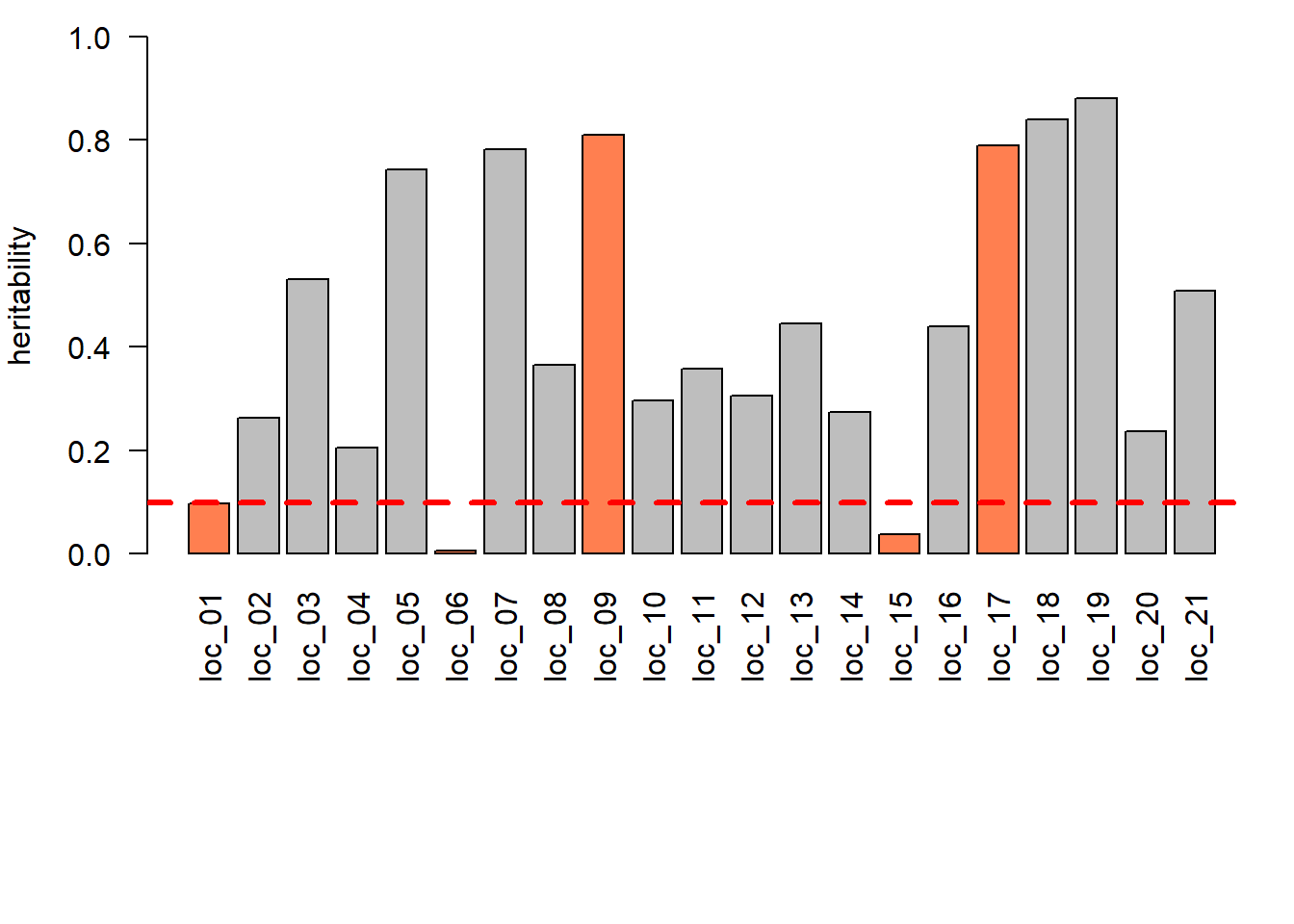
Before proceeding to step 2, a selection of trials/environments of interest is performed. In general, this corresponds to all trials relevant to the current study or analysis. As there might be several single environment analyses accumulated over time, it is possible to select these for different objectives. For example, all sites for a given breeding zone over the last three years. Or trials associated with some environmental stress (e.g., drought). A key aspect of this selection is that these trials need to be somehow connected, implying that there is a need for a group of entries to be common between trials. This is described in further detail in other sections.

A second criteria is associated with the quality of the information associated with a given trial/environment. Here, for example, it might be considered that trials with low heritability (e.g., < 0.10) might need to be dropped as they do not have sufficient genetic signal to be considered for the step 2 analysis. Several other criteria can be considered, such as average yield, residual variance (or CV%), etc. The aim is to consider a group of trials that should provide reasonable information.

It is important to note that it is also possible to select only a relevant set of genotypes; or discard some genotypes that seem poorly represented or are of no interest. For example, some controls can be left out if they do not belong to the population of interest. As indicated earlier, the only critical aspect is that there is sufficient connectivity between trials in order to have a reasonable estimate of genetic correlation between trials.

In the case presented below, there are 3 trials that were dropped given their low heritability (< 0.10), but other criteria might be considered.

# read stage-1 outputs
summS <- read.csv(paste0("outputs/", study.name, "_", trait.name, "_Stage-1_Summary_Statistics.csv"))
predS <- read.csv(paste0("outputs/", study.name, "_", trait.name, "_Stage-1_Predictions.csv"))

# explore the results from the sites
# eliminate trials with h2VC < threshold (e.g., 0.10)
valid.env <- summS[!is.na(summS$sel_model) & 
                   ((summS$Type != "AUGMENTED" & summS$heritVC > as.numeric(config$met$heritVC.limit)) |
                   (summS$Type == "AUGMENTED" & summS$Pvalue < as.numeric(config$met$Pvalue.limit))), 
                   "Environment"]

# filter to sites of interest/valid
sel.predS <- predS[predS$Environment %in% valid.env,]

excluded.loc  <- trimws(strsplit(config$met$excluded.loc, ",")[[1]])
excluded.geno <- trimws(strsplit(config$met$excluded.geno, ",")[[1]])

sel.predS <- sel.predS[!(tolower(sel.predS$Environment) %in% tolower(excluded.loc)),]
sel.predS <- sel.predS[!(tolower(sel.predS$gen) %in% tolower(excluded.geno)),]

case.color <- ifelse(!summS$Environment %in% valid.env | summS$Environment %in% excluded.loc, "coral", "gray")

if (summS$Type[1] != "AUGMENTED") {
  par(mar=c(10,4,1,1))
  barplot(summS$heritVC, ylim = c(0,1), names.arg = summS$Environment, las = 2, 
          ylab = "heritability", col = case.color)
  abline(h = as.numeric(config$met$heritVC.limit), lty = 2, lwd = 3, col = "red")
} else {
  par(mar=c(10,4,1,1))
  barplot(summS$Pvalue, ylim = c(0,1), names.arg = summS$Environment, las = 2, 
          ylab = "P-Value", col = case.color)
  abline(h = as.numeric(config$met$Pvalue.limit), lty = 2, lwd = 3, col = "red")
}

# we may also select/filter the list of geno of interest (e.g. filter out local checks)
message(paste("<b>Excluded environments in config.ini:</b>", config$met$excluded.loc,
              "<br/><b>Excluded genotypes in config.ini:</b>", config$met$excluded.geno))

Excluded environments in config.ini: loc_17, loc_09
Excluded genotypes in config.ini: geno_02, geno_11, geno_16, geno_20

Excluded sites

create_dt(summS[!(summS$Environment %in% valid.env), c("Environment", "heritVC", "Pvalue")])

5.2 Auditing Data for MET Analysis

The selected set of trials/environments to be analyzed, as indicated, needs to be audited in order to see if this set is reasonable for downstream analyses. The main aspect is related to connectivity between trials through genotypes in common. Recall that the corh and fa structure allow for poor connectivity compared to corgh and us structures.

If connectivity is poor, it is possible to eliminate some of the trials that are with limited connections (or no connections). But also, this might require splitting/separating the group of trials into two or more sets to be evaluated independently. This can be assessed better with a heatmap/clustering to separate them. In the example presented below, all genotypes are present in all sites, therefore this is an ideal set.

# auditMET object has two components
# $incidence to show/present connectivity between 
# env (in terms of shared geno #), or geno (in terms of shared env #)
# $stats simple summary statistics (n, mean, min, max, sd, and CV)
audit.Env <- auditMET(data=sel.predS, gen="gen", trial="Environment", resp="predicted.value", single=TRUE)
audit.Gen <- auditMET(data=sel.predS, gen="Environment", trial="gen", resp="predicted.value", single=TRUE)

# if there is no variation, then no valid heatmap/clustering can be generated
if (length(table(audit.Env$incidence)) != 1) {
  heatmap(audit.Env$incidence)
  heatmap(audit.Gen$incidence) 
}

5.2.1 Environment Stats

The table below presents the summary statistics by environment.

create_dt(audit.Env$stats)

5.2.2 Genotype Stats

The table below presents the summary statistics by genotype across all environment.

create_dt(audit.Gen$stats)

What to do if problems.

5.3 Model Fitting Process with FAx

The key on the step 2 from the two-stage analyses is on fitting a MET model that has a complex variance-covariance structure for the term genotype-nested-within-environment factor. This MET model is fitted by fixing the error variances (single term fixed to 1), but by considering for each prediction value its corresponding weight.

Several structures are available, but the most relevant one is factor analytic (FA), for which FA models from order 1 to order 9 are available. As the order increases, more variance components are estimated approximating better to the unstructured (us) matrix structure. However, the order will depend on the number of trials considered in the set selected.

The table below presents summary and goodness-of-fit statistics for these models. As these step 2 models only differ on their random effects, and all these models are nested with each other, the criteria to use can be either logL, AIC, or BIC. The recommendation is to use the one with the lowest logL value. But it is also possible to use sequential likelihood-ratio tests (LRT) to identify the best model. In any case, once a model is selected it is strongly recommended to assess the corresponding variance-covariance matrix (as a heatmap of genetic correlation for example as shown later) to assess its quality (and see if is biologically reasonable). In this example, an FA of order 6 was selected.

faModels <- list()
i <- 1

repeat{
  fa.model <- paste0("fa", i)
  
  try({
    faMET <- stageMET(data=sel.predS, gen="gen", trial="Environment", resp="predicted.value", weight="weight",
                      type.gen="random", type.trial="fixed", vc.model=fa.model, rotation="varimax", vcovp="TRUE")
  
    # check what output components are available
    # ls(faMET)
    faModels[[i]] <- faMET
  
    # good of fit indices and fa cum.var (can be used for criteria to exit the for loop)
    if(i > 1){
      # A test statistic equal to twice the absolute difference in these log-likelihoods
      # is assumed to be distributed as Chi square with one degree of freedom (one term 
      # of difference between the two models).
      # p.value <- 1 - pchisq(2 * (model1$loglik - model2$loglik), 1)
      # if p.value < 0.05 we would therefore conclude that the new model significantly
      # improves the fit of the previous model, given an increase in log-likelihood.
      testing.significance <- signif(1 - pchisq(2 * (as.data.frame(faMET$gfit)$logL - as.numeric(exit.criteria[i-1,'logL'])), 1), digits = 3)
      
      exit.criteria <- rbind(exit.criteria, c(faMET$gfit, tail(faMET$cum.var,1)[2], fa.model, testing.significance))
    }else{
      exit.criteria <- as.data.frame(faMET$gfit)
      exit.criteria$cum.var <- tail(faMET$cum.var,1)[2]
      exit.criteria$fa <- fa.model
      exit.criteria$p.value <- 0
    }
  })
  
  i <- i + 1
  
  if(i > 9) break
}

exit.criteria$logL <- as.numeric(exit.criteria$logL)
exit.criteria$AIC  <- as.numeric(exit.criteria$AIC)
exit.criteria$BIC  <- as.numeric(exit.criteria$BIC)

5.3.1 How ‘Best’ Model is Selected

exit.criteria

create_dt(exit.criteria)

# find the min logL (best model criteria)
if (is.na(as.numeric(config$met$best.fa))) {
  i <- which.max(exit.criteria$logL)
} else {
  i <- as.numeric(config$met$best.fa)
}

sel.model <- faModels[[i]]

Selected best model is 6

5.3.2 Interpreting Final Fitted Model

5.3.2.1 GxE correlation matrix

The heatmap below represents an illustration of the genetic correlations between trials/environments based on the selected FA model. It is important to check the range of correlation estimates. In this particular example, there are negative and positive values, and this needs to be verified with the understanding of the set of trials. This might be an indication of issues (e.g., poor connectivity or trial installation difficulties).

In the present example, it is also possible to identify 2 or 3 groups of trials (by checking dendrograms), and this can assist in separating the trials into additional sets to be analyzed independently or to assist on the definition of target population environments (TPEs).

# genetic correlation matrix between environments
# sel.model$corr.M
pheatmap(sel.model$corr.M, color = colorRampPalette(RColorBrewer::brewer.pal(n = 7, name = "RdYlBu"))(101), breaks = seq(-1, 1, by = 0.02))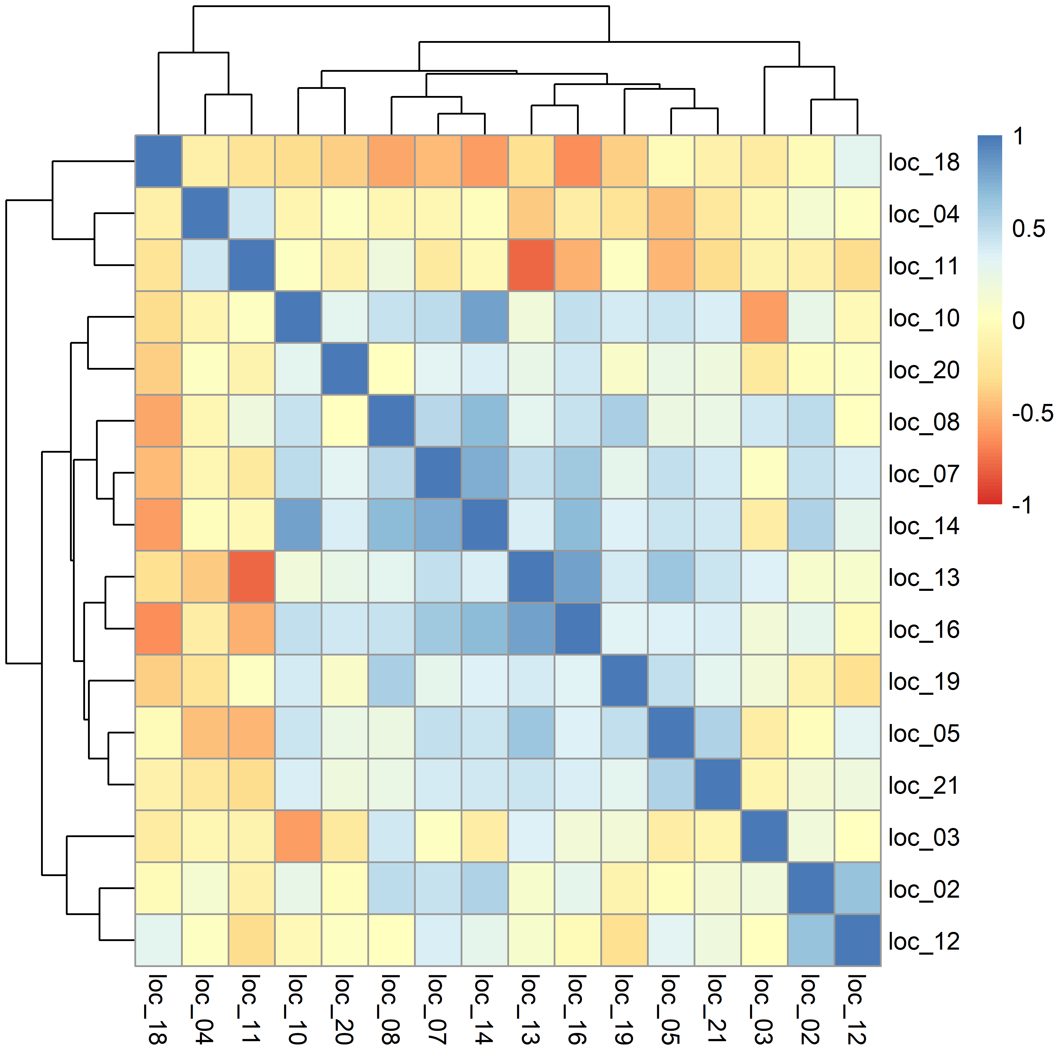

5.3.2.2 Overall Variance Explained

The variance components of the final selected FA model, here FA6, can be processed to obtain the proportion of variance explained from the complete GxE analysis. In this example, the 6 factors explain 82.1% of the total GxE variability.

create_dt(as.data.frame(sel.model$cum.var))

5.3.2.3 Variance Explained by Env.

Exploration of the individual variance components for each of the trials/environments allows for a calculation of the contribution of each factor to explain the GxE variability but in this case for each of the trials. This is presented in the table below, and it is noticed that in all trials but 3, the cumulative variance explained is larger than 70% with many trials having values close to 100%. This can lead to further understanding of the main underly environmental factors that affect the responses within a given trial.

create_dt(as.data.frame(sel.model$cum.var.site))

5.3.2.4 Predictions

The table below presents the final predictions for all entries in each of the trials with their standard error. In addition, there is an additional column that indicates if the prediction corresponds to an extrapolation, this is the case for some entries that have a prediction for trials/environments on which they were not evaluated.

Note that these are the final predictions for each entry in each trial based on the estimated variance-covariance structure selected. In addition, their standard errors will reflect the level of information available on each of these predictions. Nevertheless, it is important to consider these standard errors as approximated (and likely to be underestimated); however, their predicted values are unbiased.

It is recommended to use this table for calculating predictions across trials of interest (a subset of the ones here if these correspond to different target population environments) and to perform any downstream stability calculations to select the best entries (with broad or specific adaptability), and calculations of genetic gains.

create_dt(sel.model$predictions)

5.3.2.5 Rotate Loadings

The estimated matrix of loadings across all trials is often rotated to facilitate its interpretation. In this case, a varimax is considered by default. It is possible to associate (correlate) these rotated loadings to environmental variables by simple linear relationships for further understanding of the environmental variables driving GxE.

# n rows for sites, and m columns for fa components
# each fa loading vector may correlated with available environmental variables
# trying to find the highest correlated one that can interpret this component
# biplot technique can be used also to interpret this result
#
# sel.model$fa.loadings
# sel.model$fa.rot.loadings
create_dt(as.data.frame(sel.model$fa.rot.loadings))

5.3.2.6 Latent Regression Plots

The use of FA models with an exploration of the BLUP effects together with the factor loadings allows for a better understanding of the dynamics of GxE for a given genotype. The plots presented here can be assessed for this purpose. For example, finding if the relationship is flat (no slope) will indicate that the given genotype is not affected by the underlying factor. In contrast, strong negative or positive slopes will indicate some GxE response with large or small effects on a set of trials. A genotype with a projection of zero on the y-axis has an average response at the given trial.

latent.reg.plots <- paste("fa", expand.grid(1:i, levels(sel.model$predictions$gen))$Var1, 
                          "_",  expand.grid(1:i, levels(sel.model$predictions$gen))$Var2, 
                          sep = "")

select.latent.reg <- paste0("plots/latent_reg_", latent.reg.plots, "_", trait.name, ".png")
names(select.latent.reg) <- latent.reg.plots

bsselect(select.latent.reg, 
         type = "iframe", 
         live_search = TRUE, 
         show_tick = TRUE, 
         elementId = 'latent_reg')$prepend[[1]]$html

fa1_geno_01 fa2_geno_01 fa3_geno_01 fa4_geno_01 fa5_geno_01 fa6_geno_01 fa1_geno_03 fa2_geno_03 fa3_geno_03 fa4_geno_03 fa5_geno_03 fa6_geno_03 fa1_geno_04 fa2_geno_04 fa3_geno_04 fa4_geno_04 fa5_geno_04 fa6_geno_04 fa1_geno_05 fa2_geno_05 fa3_geno_05 fa4_geno_05 fa5_geno_05 fa6_geno_05 fa1_geno_06 fa2_geno_06 fa3_geno_06 fa4_geno_06 fa5_geno_06 fa6_geno_06 fa1_geno_07 fa2_geno_07 fa3_geno_07 fa4_geno_07 fa5_geno_07 fa6_geno_07 fa1_geno_08 fa2_geno_08 fa3_geno_08 fa4_geno_08 fa5_geno_08 fa6_geno_08 fa1_geno_09 fa2_geno_09 fa3_geno_09 fa4_geno_09 fa5_geno_09 fa6_geno_09 fa1_geno_10 fa2_geno_10 fa3_geno_10 fa4_geno_10 fa5_geno_10 fa6_geno_10 fa1_geno_12 fa2_geno_12 fa3_geno_12 fa4_geno_12 fa5_geno_12 fa6_geno_12 fa1_geno_13 fa2_geno_13 fa3_geno_13 fa4_geno_13 fa5_geno_13 fa6_geno_13 fa1_geno_14 fa2_geno_14 fa3_geno_14 fa4_geno_14 fa5_geno_14 fa6_geno_14 fa1_geno_15 fa2_geno_15 fa3_geno_15 fa4_geno_15 fa5_geno_15 fa6_geno_15 fa1_geno_17 fa2_geno_17 fa3_geno_17 fa4_geno_17 fa5_geno_17 fa6_geno_17 fa1_geno_18 fa2_geno_18 fa3_geno_18 fa4_geno_18 fa5_geno_18 fa6_geno_18 fa1_geno_19 fa2_geno_19 fa3_geno_19 fa4_geno_19 fa5_geno_19 fa6_geno_19 fa1_geno_21 fa2_geno_21 fa3_geno_21 fa4_geno_21 fa5_geno_21 fa6_geno_21 fa1_geno_22 fa2_geno_22 fa3_geno_22 fa4_geno_22 fa5_geno_22 fa6_geno_22 fa1_geno_23 fa2_geno_23 fa3_geno_23 fa4_geno_23 fa5_geno_23 fa6_geno_23

You can find the latent regression plots here

5.3.2.7 Model Call

In the present workflow, all analyses are done using ASReml-R. Given the complexity of some of the models, and future interest in exploring further the model fitted, the following objects obtained from the MET fitted in the second step provide the definition of the LMM as required for ASReml-R.

• call: String with the ASReml-R call used to fit the requested model.
• mod: ASReml-R object with all information from the fitted model.

# the whole fitted model still available to extract any further info (e.g., the full list of varcomp)
# summary(sel.model$mod)$varcomp

• vcov.M: GxE variance-covariance matrix.
• vcov.P: Variance-covariance matrix of predictions.

# calculate the genetic variance per environment (i.e., measure genetic variability in each env)
# this can be useful in site selection for example
# sqrt(diag(sel.model$vcov.M))

6 Closing Remarks

The current workflow for MET analyses as illustrated here represents a very practical and operational procedure to follow based on the state-of-the-art multi-environmental trials analysis and using the modern statistical software considering a complex variance-covariance structure, such as FA. This procedure is backed by several manuscripts and by the personal experience of the authors.

As with any workflow, this is dynamic and future advancements and use of it will allow for improvements. However, some of the elements that are currently identified as relevant in future editions are:

• Incorporation of a pedigree-based or genomic-based relationship matrix to estimate breeding values, additive x environment interaction, and narrow-sense and genomic heritabilities.

• Extensions on the graphical output and interpretation of the Biplots.

• Addition of functions for stability indexes that will assist in the selection of future entries.